We will be working with the Fashion MNIST dataset. The CSV files came from Kaggle.

The Fashion-MNIST dataset proves to be slightly more challenging than the original MNIST dataset of hand drawn 28x28 sized numbers.

I took heavy inspiration from Samson Zhang . They truly kick started my desire to learn as much about neural networks as possible link to there kaggle. Samsons guidance was very much appreciated when I first started to learn about how to make my own neural network without any fancy python libraries.

📓 This post is adapted from a Jupyter notebook. View the source on GitHub or open it in Colab.

import numpy as np
import pandas as pd
import math
from matplotlib import pyplot as plt

import kagglehub
path = kagglehub.dataset_download("zalando-research/fashionmnist")

Forward Propagation

Information on our dataset: We are working with a dataset of images where each image has 784 pixels.

Our neural network will be very simple only utilizing only 3 layers; Input, Hidden, and Output.

Input Layer

Our Input Layer is very simple. It is the image itself!

Our image has 784 pixels, each pixel holding a value from 0-255(0 = black, 255 = white).

We will feed this image into our neural network through a method known as Forward Propagation.

Hidden Layer

Hidden Layers are a bit of a mystery. Understanding how many neurons you need may be difficult. Add too many neurons and you may cause Overfitting or your training times may get extremely slow. If you do not add enough neurons you may cause some Underfitting

For now to keep it simple we will stick with using only 10 neurons so that we may focus on the important and Fun-damental parts of a neural network!

Output Layer

This is where our neural network will come to some sort of conclusions based on the probabilites that were outputted based on the mathematics previously performed!

Our output layer has 10 Classifications based on the classes provided by the Fashion-MNIST data set.

Those being: {T-shirt/Top, Trouser, Pullover, Dress, Coat, Sandal, Shirt, Sneaker, Bag, Ankle boot}

Reading the Dataset

We will begin reading and testing our dataset

data = pd.read_csv(path+"/fashion-mnist_train.csv")

Taking a Peek at Our Dataset

data.head()

   label  pixel1  pixel2  pixel3  pixel4  pixel5  pixel6  pixel7  pixel8  \
0      2       0       0       0       0       0       0       0       0   
1      9       0       0       0       0       0       0       0       0   
2      6       0       0       0       0       0       0       0       5   
3      0       0       0       0       1       2       0       0       0   
4      3       0       0       0       0       0       0       0       0   

   pixel9  ...  pixel775  pixel776  pixel777  pixel778  pixel779  pixel780  \
0       0  ...         0         0         0         0         0         0   
1       0  ...         0         0         0         0         0         0   
2       0  ...         0         0         0        30        43         0   
3       0  ...         3         0         0         0         0         1   
4       0  ...         0         0         0         0         0         0   

   pixel781  pixel782  pixel783  pixel784  
0         0         0         0         0  
1         0         0         0         0  
2         0         0         0         0  
3         0         0         0         0  
4         0         0         0         0  

[5 rows x 785 columns]

# this will show the dimensions of our dataset
data.shape

(60000, 785)

We can see that we have 60,000 rows and 785 columns.

This is good, but later we will have to transpose our data so that we can work with our images as columns.

If we were to work with the dataset without transposing:

1. It would simply be very incorrect
2. Because our dataset has 60,000 that means we have 60,000 variables corresponding to images and not actual data.

So we must transpose to work with the individual pixels and there associated variables!

Actual Coding!

We will begin by vectorizing our dataset so that we are not working directly with the csv file

data_vec = np.array(data) # this makes everything in our csv into an array

# defining Rows (m) and columns (n)
m, n = data_vec.shape
# m = 60,000 n = 785

# shuffling our data like a deck of cards
# we do this because we want to be sure that the training is on a set of random
# images each time
np.random.shuffle(data_vec)

Splitting Our Training Set

We want to split our training set. One portion will be used to for training our neural network, the other portion will be used to test.

Despite our data set providing a seperate test set, we do not want to use that test set until the very end.

Think of that last test set as the final exam for our neural network and our test set that came from splitting the training set as a midterm!

# transposing the first 1000 rows from the training file
data_dev = data_vec[0:1000].T
Y_dev = data_dev[0]
X_dev = data_dev[1:n] / 255. # Normalize pixel values to be between 0 and 1

# transposing the rest of the dataset for actual training purposes
# at this point we have a training set of 59,000 images
# this is the data we will be utilizing to update weights and biases
# in our neural network
data_train = data_vec[1000:m].T
Y_train = data_train[0]
X_train = data_train[1:n] / 255. # Normalize pixel values

Math Time!

Now that we have gotten most of the preliminary stuff out of the way, we now may dig in!

Starting with Forward Propagation

As we said before, our neural network has 3 layers. Now we will explain how each layer interacts with eachother mathematically!

Transposing Our Data

Let $A^{[0]} = X$

Where, $X = \begin{bmatrix} \cdots & x_1 & \cdots \\ \cdots & x_2 & \cdots \\ & \vdots & \\ \cdots & x_k & \cdots \\ \end{bmatrix}$

This matrix represents our original data set where ${x_1, x_2, \dots, x_n}$ represents our 60,000 rows of images, but as we stated earlier we really want this to be transposed so lets transpose it!

Let $A^{[0]} = X^T$

$X^T = \begin{bmatrix} \vdots & \vdots & & \vdots \\ x_1 & x_2 & \cdots & x_k \\ \vdots & \vdots & & \vdots \\ \end{bmatrix}$

Much better now!

This represents where we currently are in the code.

Feeding Our Matrix Through the Neural Network

To feed out images through our neural network we must define a neuron!

Neuron’s are a weighted sum plus some bias.

$Z^{[l]} = W^{[l]}X^{[l-1]}+b^{[l]}$

Since we let $A = X$ our formula becomes

$Z^{[l]} = W^{[l]}A^{[l-1]}+b^{[l]}$

Now this oddly looks exactly like another formula that we should all know and love. That is the formula for a line on a plane! $y = mx+b$. Its quite cumbersome knowing how simple some of the math is behind neural networks!

However, the intuition for them is extremely difficult to grasp.

Breaking Down Our Formula

$Z^{[n]} =$ Hidden Layer Output

$W^{[n]} =$ Weights

$b^{[n]} =$ Bias

In the beginning our Weights and Bias will be chosen at random. We will go into more detail as to how we train these weights and biases to give us more accurate predictions later down the notebook.

Finding $Z^{[1]}$ Hidden Layer Output

$Z^{[1]}$ corresponds to our first Hidden Layer output

$Z^{[1]} = W^{[1]}A^{[0]} + b^{[1]}$

Lets take a look at the dimensions of our matrices and vectors in the formula

$Z^{[1]} = dim(W^{[1]})dim(A^{[0]}) + dim(b^{[1]})$

$Z^{[1]} = (10 \times 784)(784 \times k) + (10 \times 1)$

Where $k$ is the number of images being passed through the neural network.

$= (10 \times k) + (10 \times 1)$

$Z^{[1]} = (10 \times k)$

In the end we are left with the output of our Hidden Layer matrix.

Activation Functions

Activation Functions are what makes the math non-linear meaning we are going to apply a function to our $Z^{[1]}$ output to make our linear function into something curvy so that later on we can find a nice happy little descent that will give us our (hopefully) desired answer.

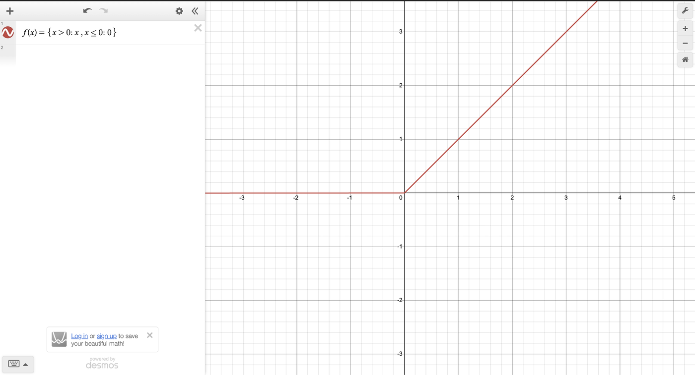
There are a few Activation Functions however, we will be dealing with ReLU (Rectified Linear Unit)

In essence we are utilizing ReLU to create a vector of non-negative numbers.

We now will apply $ReLU$,

$A^{[1]} = ReLU(Z^{[1]})$

$dim(Z^{[1]}) = dim(A^{[1]})$

Thus making our Hidden Layer output non-linear and ready for to be used for our next layer

Graph of ReLU

Finding $Z^{[2]}$ Output Layer Output

We must repeat the process similarly to how we found $Z^{[1]}$

$Z^{[2]} = W^{[2]}A^{[1]} + b^{[2]}$

$= (10 \times 10) (10 \times k) + (10 \times 1)$

$= (10 \times k)$

Thus, giving us the output of our Output Layer.

However, if we take a closer look at our output (for the time being lets assume $k = 1$ which means we are looking at a single image)

$dim(Z^{[2]}) = (10 \times 1)$

Each element within this vector will now tell us a probabiliy of what the neural network believes that the image may be classified as.

However, the results are not particualarly what we are looking for so we must normalize the vector by introducing the Softmax function

Softmax Function

The Softmax function helps us further interpret our probabilites of which classification our neural network believes that the input image may be.

$Softmax(Z^{[2]}) = \hat{y}_i = \dfrac{e^{Z_i^{[2]}}}{\sum_{j=1}^{10} e^{Z_j^{[2]}}}$

To those with a keen eye, you may have noticed that this function will normalize our data so that the sum of each element wil equal 1.

This helps us better interpret the probability of whether the image is of Trousers or of a T-shirt

We are exponentiating each element in $Z^{[2]}$ then dividing them by the exponentiation of each element summed!

If you take an even closer look you should have noticed that we are dividing by the Manhattan Norm or the $L_1$ Norm

Coding Forward Propagation!!! Finally!!!

Initializing Parameters

First we will begin by making a function that initializes our Weights and Biases

def init_params():
  # for the first layer (Hidden Layer)
  W1 = np.random.rand(10,784) - 0.5
  b1 = np.random.rand(10,1) - 0.5

  # for the second layer (Output Layer)
  W2 = np.random.rand(10,10) - 0.5
  b2 = np.random.rand(10,1) - 0.5
  return W1, b1, W2, b2

In the beginning we want our Weights and Biases to have some values. So we choose them to have random values between $[0,1]$.

Example of what the first line in the funciton is doing

W1 Has 10 rows 784 columns where each element is a random value sitting between 0 and 1

Since we are subtracting by 0.5 we are shifting each element to be centered around 0

If our smallest element is 0 then $0 - 0.5 = -0.5$

If our largest element is 1 then $1 - 0.5 = 0.5$

Therefore, our new interval for all numbers are between $[-0.5,0.5]$

We want this as when we apply our Activation Function we can ignore the values that are negative, the negative values imply that the neural network believes theyre strongly not a part of that classification.

Activation Functions

Before we begin our Forward Propagation We need to create our Activation Functions

# this is precisely what we defined earlier
# we compare each element to 0
# x, x > 0
# 0, x <=0


#def relu(Z):
#  return np.maximum(0,Z)

Testing Wtih GELU

Recently I had learned about Gaussian Error Linear Unit and from what we understand is that GELU acts as a better activation function in comparison to RELU. This mostly comes from the idea that it does not compeletely kill the neurons when they fire. However, this allows them to introduce some thought and skew the results slightly more.

$GELU(x) =0.5 \cdot x \cdot \left( 1 + \tanh\left( \sqrt{ \dfrac{2}{\pi} } \cdot (x + 0.44715) * x^3 \right) \right)$

def gelu(Z):
  return 0.5 * Z * (1 + np.tanh(np.sqrt(2 / np.pi) * (Z + 0.044715 * Z ** 3)))

Softmax Function

This is our softmax function. Again, This will make every sit somewhere between $[0,1]$ where the sum of all elements after the softmax function is applied is equal to $1$

# exactly how we defined our softmax function previously
def softmax(Z):
  # Subtract max for numerical stability to prevent overflow
  Z = Z - np.max(Z, axis=0, keepdims=True)
  A = np.exp(Z) / np.sum(np.exp(Z), axis=0, keepdims=True)
  return A

Forward Propagation

This is where we tie everything together and how feeding our image through the neural network works.

def forward_prop(W1, b1, W2, b2, X):
  # output of our first layer (Hidden Layer)
  Z1 = W1.dot(X) + b1

  # making our output non-linear using ReLU
  #A1 = relu(Z1)

  # making our output non-linear using GeLU
  A1 = gelu(Z1)

  # feeding our non-linear A1 to the next layer (Output Layer)
  Z2 = W2.dot(A1) + b2

  # using softmax to truly determine what the neural network believes
  # the image may be classified as at the moment
  A2 = softmax(Z2)
  return Z1, A1, Z2, A2

This is how the math looks for the forward_prop function

After the Softmax Our vector of a single image passing through the Forward Propagation will look something like this

At the moment all we have is some random prediction. We do not know if it is correct at, so we must implement a Cost Function

One-Hot Encoding

One-Hot Encoding is a method for converting categorical labels such as {T-shirt/Top, Boots, ..., etc.}into quantative data so that it may be processed by our neural network.

We set our vectors elements all to $0$ however, we leave one element set to $1$ to represent where in the classifier list we are at.

For example, say we are dealing with an image of {Boots} then our vector will look like:

$\begin{bmatrix} 0 & 1 & 0 & 0 & 0 & 0 & 0 & 0 & 0 & 0 & 0 \end{bmatrix}$

The columns represent our Classification and the rows represent the number of images inputted.

We then transpose the vector so that we may be able to do math more easily with it.

$Y \rightarrow Y_{One-Hot}: \begin{bmatrix} 0 \\ 1 \\ 0 \\ 0 \\ 0 \\ 0 \\ 0 \\ 0 \\ 0 \\ 0 \\ \end{bmatrix}$

def one_hot(Y):

  # here we create a matrix full of 0
  # rows = Y.size
  # cols = Y.max() + 1 = 10
  one_hot_Y = np.zeros((Y.size, Y.max() + 1 ))

  # This is how we will set an element in the matrix to 1
  # np.arange takes in number of images = y.size
  # then this line will go through to every row at column Y
  # and set that element to 1 to represent what that row will
  # classified as
  one_hot_Y[np.arange(Y.size), Y] = 1

  return one_hot_Y.T

Backpropagation

“Backpropagation is a gradient computation method commonly used for training neural networks in computing parameter updates”

After our first Forward pass the corresponding output will mostlikely be incorrect as we had choosen random elements for the Weights and Biases vectors.

Doing this Backpropagation method is what will give us more accurate results as we will now be updating our Weights and Biases through each pass.

Underlying Math for Backpropagation

Backpropagation allows for us to understand how the weights and the biases in a neural network change in order to make more accurate predictions as training continues.

We change these weights and biases by computing derivatives via the chain rule and Gradien Descent.

How Backprop Algorithm Works

When building our backpropagation algorithm, we care about three things: Error in our Output Layers $Z^{[1]},Z^{[2]}$ the weights and biases associated with that layer $W^{[1]},W^{[2]},b^{[1]},b^{[2]}$

The computation to find the derivatives are a little invloved, for now we will skipe them. However, if you desire to see them the following material helped me understand them from mathematics stand point:

The Matrix Calculus You Need For Deep Learning

The Complete Mathematics of Neural Networks and Deep Learning

How the backpropagation algorithm works

An Overview Of Artificial Neural Networks for Mathematicians

Output layer Gradients

Error of $dZ^{[2]}$:

Weights Gradient $dW^{[2]}$:

Bias Gradient $dW^{[2]}$:

ReLU Derivative

Let us take a look back at our Activation Function.

More clearly we see that when $x > 0 \rightarrow f(x) = x$ and $x \leq 0 \rightarrow f(x) = 0$

Therefore, the derivative of the functions comprising $ReLU$ are trivial.

$f'(x) = 1, \qquad f'(x) = 0$

# if an element in Z is greater than 0
# return 1 else return 0
#def relu_deriv(Z):
#  return Z > 0

Testing GELU derivative

def gelu_deriv(Z):
  return 0.5 * (1 + np.tanh(np.sqrt(2 / np.pi) * (Z + 0.044715 * Z ** 3)))

Hidden Layer Gradients

Error of $dZ^{[1]}$:

Weights Gradient $dW^{[1]}$:

Bias Gradient $dW^{[2]}$:

Backprop Code

def back_prop(Z1, A1, Z2, A2, W1, W2, X, Y):
  m = Y.size # batch size

  # calling our one_hot function
  one_hot_Y = one_hot(Y)

  # our output layer error
  #
  # predicted probabilities minus our One-Hot vector
  # the difference between what the network predicted and the actual answer
  dZ2 = A2 - one_hot_Y

  # we take the error and multiply it by the input that created it
  # then we transpose so the the multiplication works
  dW2 = 1 / m * dZ2.dot(A1.T)

  # since the bias is added to every single example in the batch its gradient
  # is the avg of the errors from all examples
  # Sum across the batch (axis 1) to get a column vector
  db2 = 1 / m * np.sum(dZ2, axis=1, keepdims=True)

  # our hiddent layer error
  #
  # these lines do the same thing however this time we now also must find
  # derivative of ReLU
  # the derivative of ReLU essentially gets rid of the gradient if Z1 < 0
  # this tells us that that it had no contribution towards our prediction
  #
  # later talk about how negative probability means the neural net thinks that
  # that element had 0 contribution in determining what the classification of
  # the image is
  #dZ1 = W2.T.dot(dZ2) * relu_deriv(Z1)

  dZ1 = W2.T.dot(dZ2) * gelu_deriv(Z1)

  dW1 = 1 / m * dZ1.dot(X.T)
  db1 = 1 / m * np.sum(dZ1, axis=1, keepdims=True)

  return dW1, db1, dW2, db2

Updating Parameters

These are our Loss Functions this part and the functions with it get updated after we execute our gradient descent function.

$α$ is our learning rate.

In essnence,

• higher the learning rate the faster the convergence rate
  • decreases computation time
  • you may overshoot your weights, thus giving you incorrect results
• lower the learning rate the slower the convergence rate
  • increases computation time, but it can improve accuracy

Therefore, we really want a happy medium so that the convergence and the accuracy work well for what we need!

def update_param(W1, b1, W2, b2, dW1, db1, dW2, db2, alpha):
  W1 = W1 - alpha * dW1
  b1 = b1 - alpha * db1
  W2 = W2 - alpha * dW2
  b2 = b2 - alpha * db2
  return W1, b1, W2, b2

Getting Predictions and accuracy

def get_predictions(A2):
  return np.argmax(A2, 0)

def get_accuracy(predictions, Y):
  print(predictions, Y)
  return np.sum(predictions == Y) / Y.size

Gradient Descent

def grad_descent(X, Y, alpha, iterations):
  # here we recal that init_params() makes our starting weights and biases
  # random
  W1, b1, W2, b2 = init_params()

  # we iterate over every image by feeding it to our
  #   forward prop
  #   back prop
  # then lastly we update our weights and biases so that during our next iteration
  # we get more accurate results
  for i in range(iterations):
    Z1, A1, Z2, A2 = forward_prop(W1, b1, W2, b2, X)
    dW1, db1, dW2, db2 = back_prop(Z1, A1, Z2, A2, W1, W2, X, Y)
    W1, b1, W2, b2 = update_param(W1, b1, W2, b2, dW1, db1, dW2, db2, alpha)

    # printing the prediction after every 10 iterations
    if i % 10 == 0:
      print("Iteration: ", i)
      print("")
      predictions = get_predictions(A2)
      print(get_accuracy(predictions, Y))

  return W1, b1, W2, b2

W1, b1, W2, b2 = grad_descent(X_train, Y_train, 0.10, 500)

Iteration:  0

[6 9 6 ... 8 8 9] [7 0 1 ... 9 1 0]
0.112
Iteration:  10

[8 9 1 ... 9 3 4] [7 0 1 ... 9 1 0]
0.32308474576271184
Iteration:  20

[8 8 1 ... 9 1 4] [7 0 1 ... 9 1 0]
0.4609322033898305
        [... 44 iterations omitted ...]

Iteration:  480

[8 2 1 ... 9 1 0] [7 0 1 ... 9 1 0]
0.7420847457627119
Iteration:  490

[8 2 1 ... 9 1 0] [7 0 1 ... 9 1 0]
0.7432372881355932

Our Models Accuracy on the training set

It looks like our model is $\approx 75\%$ accurate in accordance to our training set

class_names = [
    "T-shirt/top", "Trouser", "Pullover", "Dress", "Coat",
    "Sandal", "Shirt", "Sneaker", "Bag", "Ankle boot"
]

def make_predictions(X, W1, b1, W2, b2):
    _, _, _, A2 = forward_prop(W1, b1, W2, b2, X)
    predictions = get_predictions(A2)
    return predictions

def test_prediction(index, W1, b1, W2, b2):
    current_image = X_train[:, index, None]
    prediction = make_predictions(X_train[:, index, None], W1, b1, W2, b2)
    label = Y_train[index]

    print("Prediction: ", class_names[prediction[0]])
    print("Label: ", class_names[label])

    current_image = current_image.reshape((28, 28)) * 255
    plt.gray()
    plt.imshow(current_image, interpolation='nearest')
    plt.show()

test_prediction(0, W1, b1, W2, b2)
test_prediction(1, W1, b1, W2, b2)
test_prediction(2, W1, b1, W2, b2)
test_prediction(3, W1, b1, W2, b2)
test_prediction(4, W1, b1, W2, b2)
test_prediction(5, W1, b1, W2, b2)
test_prediction(6, W1, b1, W2, b2)
test_prediction(7, W1, b1, W2, b2)
test_prediction(8, W1, b1, W2, b2)
test_prediction(9, W1, b1, W2, b2)

Prediction:  Bag
Label:  Sneaker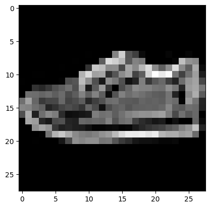

Prediction:  Pullover
Label:  T-shirt/top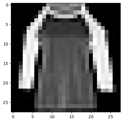

Prediction:  Trouser
Label:  Trouser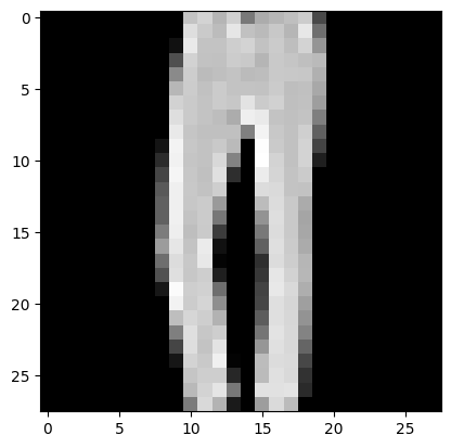

Prediction:  Shirt
Label:  Shirt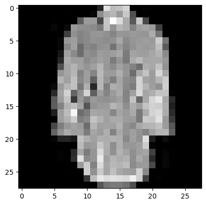

Prediction:  Ankle boot
Label:  Ankle boot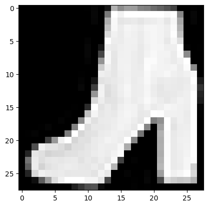

Prediction:  Sneaker
Label:  Sandal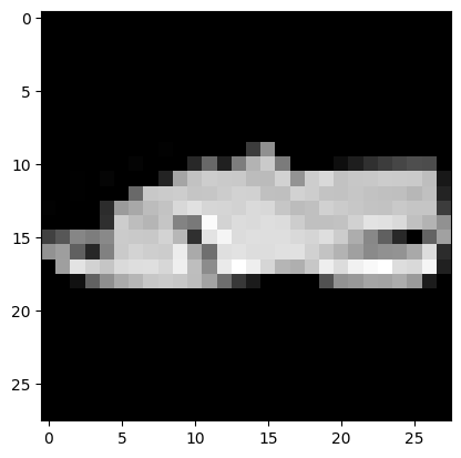

Prediction:  Sandal
Label:  Sandal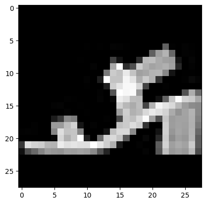

Prediction:  Coat
Label:  Coat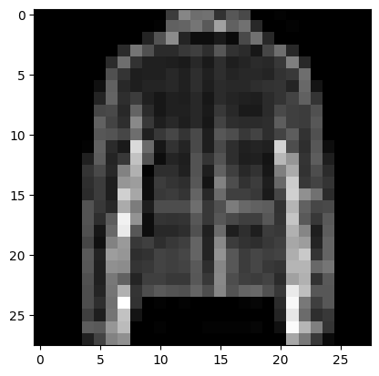

Prediction:  Sandal
Label:  Sandal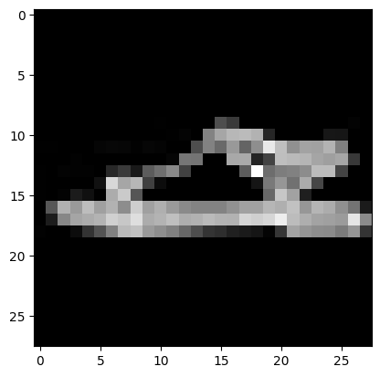

Prediction:  T-shirt/top
Label:  T-shirt/top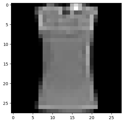

Testing our Test Set

dev_predictions = make_predictions(X_dev, W1, b1, W2, b2)
get_accuracy(dev_predictions, Y_dev)

[3 1 2 1 2 1 0 5 0 2 2 0 6 2 2 9 2 7 3 8 4 0 4 6 0 7 9 0 6 8 4 0 0 0 6 1 8 ...]

np.float64(0.744)

Therefore, our CNN is $\approx 75 \%$ accurate

Confusion Matrix Analysis

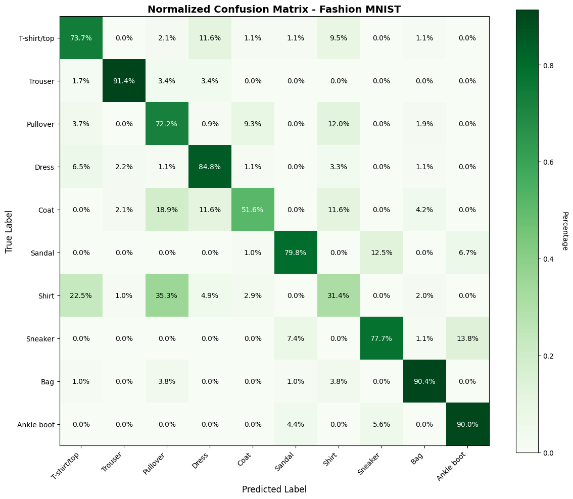
A confusion matrix helps us understand where our model is making mistakes. Each row represents the actual class, and each column represents the predicted class.

Key Metrics

Recall (aka Sensitivity)

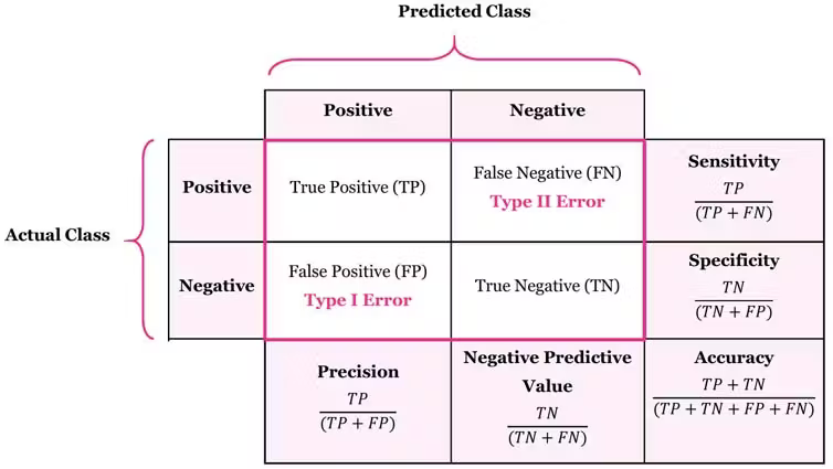
• Example: 85 found out of 100 actual Sneakers = 85% Recall

• Matters for: Medical diagnosis (can’t miss diseases), search engines (find all results)

Precision

• When we predict Sneaker, how often are we correct?

• Example: 85 correct out of 90 Sneaker predictions = 94.4% Precision

• Matters for: Spam filters (don’t block good emails), recommendations (be accurate)

F1 Score

$F1 = 2 \times \frac{\text{Precision} \times \text{Recall}}{\text{Precision} + \text{Recall}}$

• What’s the balance between precision and recall?

• Penalizes extreme values. If either metric is low, F1 is low.

Tradeoff

from sklearn.metrics import confusion_matrix

cm = confusion_matrix(Y_dev, dev_predictions)

# using matplotlib's subplots for the 10 Classes
fig, ax = plt.subplots(figsize=(12, 10))
im = ax.imshow(cm, cmap='Blues')

# plotting stuffs
cbar = plt.colorbar(im, ax=ax)
cbar.set_label('Count', rotation=270, labelpad=20)

# ticks and labels
ax.set_xticks(np.arange(len(class_names)))
ax.set_yticks(np.arange(len(class_names)))
ax.set_xticklabels(class_names, rotation=45, ha='right')
ax.set_yticklabels(class_names)

for i in range(len(class_names)):
    for j in range(len(class_names)):
        text = ax.text(j, i, cm[i, j], ha="center", va="center", color="black" if cm[i, j] < cm.max()/2 else "white")

ax.set_xlabel('Predicted Label', fontsize=12)
ax.set_ylabel('True Label', fontsize=12)
ax.set_title('Confusion Matrix - Fashion MNIST', fontsize=14, fontweight='bold')
plt.tight_layout()
plt.show()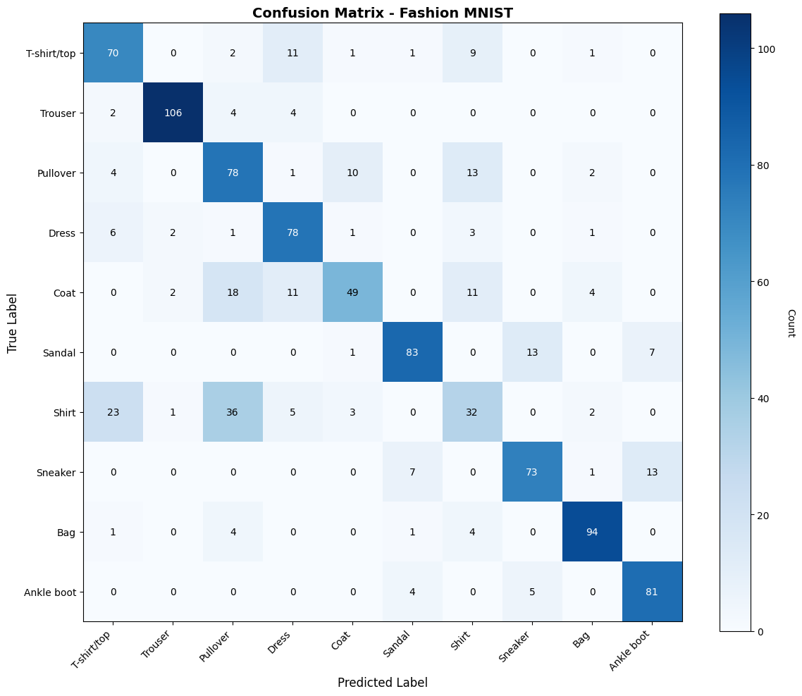

From the confusion matrix:

• Recall = diagonal value / row sum (how many actual items we found)
• Precision = diagonal value / column sum (how often predictions are correct)

# normalize confusion matrix (percentages)
cm_normalized = cm.astype('float') / cm.sum(axis=1)[:, np.newaxis]

fig, ax = plt.subplots(figsize=(12, 10))
im = ax.imshow(cm_normalized, cmap='Greens')

# Plotting stuff
cbar = plt.colorbar(im, ax=ax)
cbar.set_label('Percentage', rotation=270, labelpad=20)

# ticks and labels
ax.set_xticks(np.arange(len(class_names)))
ax.set_yticks(np.arange(len(class_names)))
ax.set_xticklabels(class_names, rotation=45, ha='right')
ax.set_yticklabels(class_names)

# text annotations e.g. percentages
for i in range(len(class_names)):
    for j in range(len(class_names)):
        text = ax.text(j, i, f'{cm_normalized[i, j]:.1%}', ha="center", va="center",
                      color="black" if cm_normalized[i, j] < 0.5 else "white")

ax.set_xlabel('Predicted Label', fontsize=12)
ax.set_ylabel('True Label', fontsize=12)
ax.set_title('Normalized Confusion Matrix - Fashion MNIST', fontsize=14, fontweight='bold')
plt.tight_layout()
plt.show()